The Pivot tool more or less does the reverse of the Transpose tool
Configuration
Select Column(s) to Hold Constant
Select the column(s) to hold constant. You can imagine that the columns you select here will remain on rows.
Select Header Column
Select the column you want to transform into columns. You can only select a single column.
Select Value Column
Select the column you want to fill into the values of the column selection you made in Step #2. You can only select a single column.
Select Aggregation
Select how you want to aggregation your value column selection from Step #3.You can choose from the following types of aggregations:
- Sum: summarize numeric values (numeric columns only)
- Average: find the average of numeric values (numeric columns only)
- Min: find the smallest numeric value (numeric and datetime columns only)
- Max: find the largest numeric value (numeric and datetime columns only)
- Count: count the occurances
- Count Distinct: count the unique occurances
- First: get the first value in the group
- Last: get the last value in the group
- Concatenate: get all your string values in a comma-separated cell (text columns only)
- Standard Deviation: find the standard deviation (numeric columns only)
- Variance: find the variance (numeric columns only)
- Median: find the median (numeric columns only)
- Skewness: find the skewness (numeric columns only)
- Kurtosis: find the kurtosis (numeric columns only)
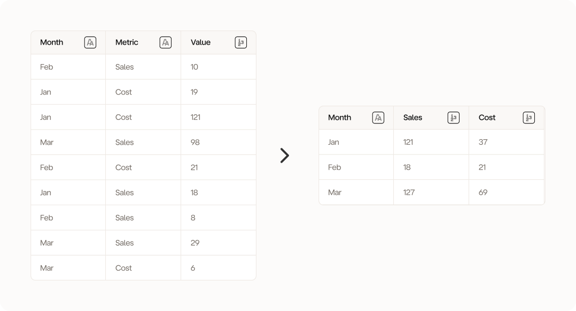
Example: The illustration example 👆
We want to pivot our data so our Metric row becomes columns and summarize the Value column per metric. We want to keep our Month constant